3.3.1 Matrix Definition & Notation
A representation of a linear transformations with components as constant multipliers. It can be used to represent a system of lines, points, or angles of rotation.
$$
A=
\begin{bmatrix}
A_{11} & A_{12} \\
A_{21} & A_{22}
\end{bmatrix}
$$
The elements by themselves are represented with $A_{ij}$
3.3.2 Identity Matrix
The matrix form of the
multiplicative identity. The diagonal from top left to bottom right is called the (as in only) diagonal, and its sum is called a trace.
$$
M\cdot M^{-1}=I=
\begin{bmatrix}
1 & 0 \\
0 & 1
\end{bmatrix}
$$
3.3.3 Matrix Arithmetic
Addition & Subtraction
Matrices may be added only if they have the same dimensions. Matrix addition and subtraction
commutes and
associates.
$$
A\pm B=
\begin{bmatrix}
A_{11}\pm B_{11} & A_{12}\pm B_{12} \\
A_{21}\pm B_{21} & A_{22}\pm B_{22}
\end{bmatrix}
$$
Product
Matrices may be multiplied regardless of dimensions (as in the starting pattern below), with the dimensions of the product being $A_{ij}\cdot B_{kl}=C_{il}$. Matrix multiplication does not
commute.
$$A\cdot B=$$
$$
\begin{bmatrix}
A_{11}\cdot B_{11}+A_{12}\cdot B_{21} & A_{11}\cdot B_{12}+A_{12}\cdot B_{22} \\
A_{21}\cdot B_{11}+A_{22}\cdot B_{21} & A_{21}\cdot B_{12}+A_{22}\cdot B_{22}
\end{bmatrix}
$$
Scalar Matrix
A number $n$ by itself is called a scalar value, and can be converted to a square matrix with the
identity matrix $n\cdot I$
$$
n→
\begin{bmatrix}
n & 0 \\
0 & n
\end{bmatrix}
$$
Scalar Distribution
Scalar coefficients
distribute throughout
$$
n\cdot A=
\begin{bmatrix}
n\cdot A_{11} & n\cdot A_{12} \\
n\cdot A_{21} & n\cdot A_{22}
\end{bmatrix}
$$
Proof of Scalar Distribution
$$
n\cdot B=
\begin{bmatrix}
n & 0 \\
0 & n
\end{bmatrix}
\cdot
\begin{bmatrix}
B_{11} & B_{12} \\
B_{21} & B_{22}
\end{bmatrix}
=
$$
$$
\begin{bmatrix}
n\cdot B_{11}+0\cdot B_{21} & n\cdot B_{12}+0\cdot B_{22} \\
0\cdot B_{11}+n\cdot B_{21} & 0\cdot B_{12}+n\cdot B_{22}
\end{bmatrix}
$$
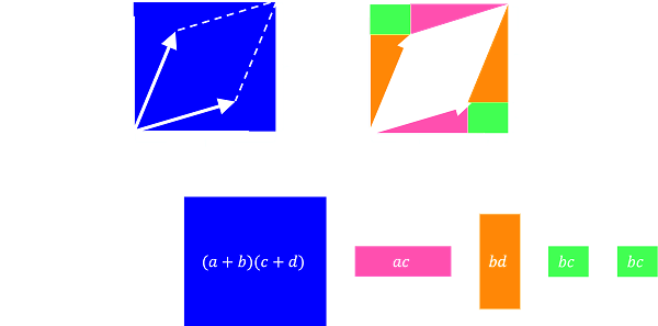
3.3.4 Determinant
The change in area when an
identity matrix undergoes linear transformation to arrive at a matrix
$$
\text{det}
\begin{bmatrix}
a & c \\
b & d
\end{bmatrix}
=
\begin{vmatrix}
a & c \\
b & d
\end{vmatrix}
=a\cdot d-b\cdot c
$$
3.3.5 Matrix Solutions with Determinants (Cramer's Rule)
Given a system of equations
$$
\begin{bmatrix}
\begin{array}{cc|c}
x_1 & y_1 & c_1 \\
x_2 & y_2 & c_2
\end{array}
\end{bmatrix}
$$
Intersections can be solved using the determinant with determinants where the solutions column becomes the transformation for that variable
$$
D\phantom{x}=
\begin{vmatrix}
\begin{array}{cc}
x_1 & y_1 \\
x_2 & y_2
\end{array}
\end{vmatrix}
\qquad
\phantom{x=\frac{Dx}{D}}
$$
$$
Dx=
\begin{vmatrix}
\begin{array}{cc}
c_1 & y_1 \\
c_2 & y_2
\end{array}
\end{vmatrix}
\qquad
x=\frac{Dx}{D}
$$
$$
Dy=
\begin{vmatrix}
\begin{array}{cc}
x_1 & c_1 \\
x_2 & c_2
\end{array}
\end{vmatrix}
\qquad
y=\frac{Dy}{D}
$$
3.3.6 Inverse Matrix
$$
A^{-1}=
\begin{bmatrix}
x_1 & y_1 \\
x_2 & y_2
\end{bmatrix}^{-1}
=
\frac{1}{\text{det}(A)}\cdot
\begin{bmatrix}
y_2 & -y_1 \\
-x_2 & x_1
\end{bmatrix}
$$
Properties
-
Inverse matrices are the result of square matrices only
-
Inverse matrices only exist when $M\cdot M^{-1}=M^{-1}\cdot M=I$
-
For a matrix to have an inverse, the determinant must not be 0
-
Inverse matrices must have determinants that are also inverses of each other; $\text{det}(M)=\text{det}(M)^{-1}$
-
$(A\cdot B)^{-1}=B^{-1}\cdot A^{-1}$
Proof by Standard Inversion
Join $A$ with $I$
$$
\begin{bmatrix}
\begin{array}{cc|cc}
x_1 & y_1 & 1 & 0 \\
x_2 & y_2 & 0 & 1
\end{array}
\end{bmatrix}
$$
Multiply row 1 by $1/x_1$
$$
\begin{bmatrix}
\begin{array}{cc|cc}
1 & y_1/x_1 & 1/x_1 & 0 \\
x_2 & y_2 & 0 & 1
\end{array}
\end{bmatrix}
$$
Subtract row 1 multiplied by $x_2$ from row 2
$$
\begin{bmatrix}
\begin{array}{cc|cc}
1 & y_1/x_1 & 1/x_1 & 0 \\
0 & y_2-x_2\cdot y_1/x_1 & -x_2/x_1 & 1
\end{array}
\end{bmatrix}
$$
Factor and rewrite $A_{22}$
$$y_2-\frac{x_2\cdot y_1}{x_1}=\frac{x_1\cdot y_2-x_2\cdot y_1}{x_1}→\frac{\text{det}(A)}{x_1}$$
Multiply row 2 by $x_1/\text{det}(A)$
$$
\begin{bmatrix}
\begin{array}{cc|cc}
1 & y_1/x_1 & 1/x_1 & 0 \\
0 & 1 & -x_2/\text{det}(A) & x_1/\text{det}(A)
\end{array}
\end{bmatrix}
$$
Subtract row 2 multiplied by $y_1/x_1$ from row 1
$$
\begin{bmatrix}
\begin{array}{cc|cc}
1 & 0 & 1/x_1+x_2\cdot y_1/\big(x_1\cdot \text{det}(A)\big) & -y_1/\text{det}(A) \\
0 & 1 & -x_2/\text{det}(A) & x_1/\text{det}(A)
\end{array}
\end{bmatrix}
$$
Simplify $A^{-1}_{11}$
$$\frac{1}{x_1}+\frac{x_2\cdot y_1}{x_1\cdot \text{det}(A)}=$$
$$\frac{\text{det}(A)}{x_1\cdot \text{det}(A)}+\frac{x_2\cdot y_1}{x_1\cdot \text{det}(A)}=$$
$$\frac{x_1\cdot y_2-x_2\cdot y_1+x_2\cdot y_1}{x_1\cdot \text{det}(A)}=\frac{y_2}{\text{det}(A)}$$
Unjoin $I$ from $A^{-1}$, and factor out $\text{det}(A)$
3.3.7 Transpose Matrix
A matrix that's been flipped about its trace
$$
M=
\begin{bmatrix}
M_{11} & M_{12} \\
M_{21} & M_{22}
\end{bmatrix}
\qquad
M^T=
\begin{bmatrix}
M_{11} & M_{21} \\
M_{12} & M_{22}
\end{bmatrix}
$$
Properties
-
$\text{det}(M)=\text{det}(M^T)$
-
When $M^T=M$, the matrix is diagonalized
-
When $M^T=-M$, the matrix is antisymmetric
-
$M^*$ indicates a complex conjugated and transposed matrix, called a conjugate transpose
-
When $M=M^{*}$, the matrix is Hermitian, $M^H$
-
When $M=-M^{*}$, the matrix is skew-Hermitian, often written as $M^H=-M$, although intuitively it should be $M^{-H}$
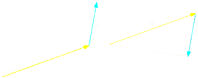
3.3.8 Vector Definition & Notation
A number with a direction and magnitude
$$\vec{v}=\lang v_x,v_y\rang=v_x\hat{\text{i}}+v_y\hat{\text{j}}$$
Properties
-
$\hat{\text{i}},\hat{\text{j}}$ are coordinate unit vectors along the $x,y$ axis
-
If the magnitude of a vector is zero, then the vector points in all directions
-
Vector components are added because they are the sum of their parts along coordinates. $v_x\hat{\text{i}}+v_y\hat{\text{j}}$ differs from common variables, i.e. $x+y$, because of their defined orthogonal nature to each other.
3.3.9 Vector Arithmetic
All
fundamental properties and
distribution apply to vectors
Addition & Subtraction
$$
\vec{u}
\pm
\vec{v}
=
\lang
\vec{u}_x
\pm
\vec{u}_y
,
\vec{v}_x
\pm
\vec{v}_y
\rang
$$
Distributive Property
$$c\cdot\vec{v}=\lang c\cdot v_x,c\cdot v_y\rang$$
3.3.A Vector Magnitude & Unit Vector
For a vector positioned at the origin
$$\|\vec{v}\|=\sqrt{v_x^2+v_y^2}$$
For a vector positioned at points $\lang x_1,y_1\rang$ leading to points $\lang x_2,y_2\rang$
$$\|\vec{v}\|=\sqrt{(x_2-x_1)^2+(y_2-y_1)^2}$$
Vector components can be determined with magnitude
$$\vec{v}=\lang\|\vec{v}\|\cdot\cos(∡0,\vec{v})\thinspace,\|\vec{v}\|\cdot\sin(∡0,\vec{v})\rang$$
A vector $\vec{u}$ at the origin with a length of 1 parallel to vector $\vec{v}$ is its unit vector
$$\pm\vec{u}=\pm\frac{\vec{v}}{\|\vec{v}\|}$$
3.3.B Dot Product
Coordinate Unit Vectors
$$\hat{\text{i}}\cdot\hat{\text{i}}=\hat{\text{j}}\cdot\hat{\text{j}}=1$$
Geometry
$$\vec{u}\parallel\vec{v}\medspace\text{ if }\medspace\vec{u}\cdot\vec{v}=\pm\|\vec{u}\|\cdot \|\vec{v}\|$$
$$\vec{u}\perp\vec{v}\medspace\text{ if }\medspace\vec{u}\cdot\vec{v}=0$$
$$\lor\medspace\|\vec{u}\|=0\medspace\lor\medspace\|\vec{v}\|=0$$
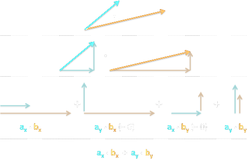
Algebraic Definition
$$\vec{u}\cdot\vec{v}=u_x\cdot v_x+u_y\cdot v_y$$
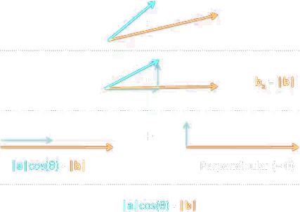
Geometric Definition
$$\vec{u}\cdot\vec{v}=\|\vec{u}\|\cdot\|\vec{v}\|\cdot\cos(∡\vec{u},\vec{v})$$
Magnitude Using Dot Product
$$\|\vec{u}\|=\sqrt{\vec{u}\cdot\vec{u}}$$
3.3.C Orthogonal Projection 🔧
The scalar component of $\vec{u}$ in the direction of $\vec{v}$
$$\text{scal}_\text{v}\text{u}=\|\vec{u}\|\cdot\cos(∡\vec{u},\vec{v})=\frac{\vec{u}\cdot\vec{v}}{\|\vec{v}\|},\medspace\vec{v}\ne 0$$
The orthogonal projection of $\vec{u}$ onto $\vec{v}$
$$\text{proj}_\text{v}\text{u}=\|\vec{u}\|\cdot\cos(∡\vec{u},\vec{v})\cdot\bigg(\frac{\vec{v}}{\|\vec{v}\|}\bigg),\medspace\vec{v}\ne 0$$
Using the scalar component for orthogonal projection
$$\text{proj}_\text{v}\text{u}=\text{scal}_\text{v}\text{u}\cdot\bigg(\frac{\vec{v}}{\|\vec{v}\|}\bigg)=\bigg(\frac{\vec{u}\cdot\vec{v}}{\vec{v}\cdot\vec{v}}\bigg)\cdot\vec{v},\medspace\vec{v}\ne 0$$
3.3.D Matrix-Vector Multiplication 🔧